(2) IMU processing 파트 중요 코드 정리
1. IMU - fast prediction
- imu_callback()
... estimator.inputIMU(t, acc, gyr); ...- imu message로부터 time (second), linear_acceleration (x,y,z), angular_velocity(roll,pitch,yaw)를 얻어서 inputIMU에 넣는다.
- imu message로부터 time (second), linear_acceleration (x,y,z), angular_velocity(roll,pitch,yaw)를 얻어서 inputIMU에 넣는다.
- void inputIMU(double t, const Vector3d &linearAcceleration, const Vector3d &angularVelocity)
if (solver_flag == NON_LINEAR) { fastPredictIMU(t, linearAcceleration, angularVelocity); pubLatestOdometry(latest_P, latest_Q, latest_V, t); }- accBuf와 gyrBuf에 각각 값을 넣어준 다음, initial이 아닌 경우 fastPredictIMU, pubLatestOdometry(단순 fastPredictIMU로부터의 odometry publish)를 수행한다. 이를통해, 이곳에서는 IMU odometry를 topic으로 쏴주는 것이고, image에 적용할 값들은 pre-integration으로 계산한다.
- accBuf와 gyrBuf에 각각 값을 넣어준 다음, initial이 아닌 경우 fastPredictIMU, pubLatestOdometry(단순 fastPredictIMU로부터의 odometry publish)를 수행한다. 이를통해, 이곳에서는 IMU odometry를 topic으로 쏴주는 것이고, image에 적용할 값들은 pre-integration으로 계산한다.
- void fastPredictIMU(double t, Vector3d linear_acceleration, Vector3d angular_velocity)
Eigen::Vector3d un_acc_0 = latest_Q * (latest_acc_0 - latest_Ba) - g; Eigen::Vector3d un_gyr = 0.5 * (latest_gyr_0 + angular_velocity) - latest_Bg; latest_Q = latest_Q * Utility::deltaQ(un_gyr * dt); Eigen::Vector3d un_acc_1 = latest_Q * (linear_acceleration - latest_Ba) - g; Eigen::Vector3d un_acc = 0.5 * (un_acc_0 + un_acc_1); latest_P = latest_P + dt * latest_V + 0.5 * dt * dt * un_acc; latest_V = latest_V + dt * un_acc; latest_acc_0 = linear_acceleration; latest_gyr_0 = angular_velocity;-
IMU linear acceleration값은 gravity값을 포함한 값도 들어오게 된다. 따라서 p,v,q는 다음과 같이 bias와 gravity를 빼준 값을 계산하게 된다.
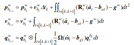
코드에서 integral 부분의 경우 평균값으로 추정하여 계산하였다.
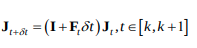
여기서 t는 현재 IMU가 들어온 frame, \(b_k\)는 이전 image에서의 IMU frame으로 보는 것이 타당하다. 즉, 쿼터니언은 k+1번째 image에서의 쿼터니언을 world frame 기준으로 구할때, k번째 image에서의 쿼터니언과 k~k+1 사이의 \(\dot{q}\)을 계산하여 integral 하여 곱해주는 것으로 계산된다.
주목할 것은 \(\dot{q}\)을 계산할때 \(b_k\)를 기준으로 계산한다는 것이다. 즉, 기준을 \(b_k\)(k번째 image에서의 imu frame)로 계산하는 것이다. 기존값들은 축적해 온것이기 때문에 world frame으로 되어 있으나 integral 안에서는 \(b_k\) frame을 기준으로 계산되기 때문. Rotation matrix를 곱할때 frame변환을 하게되고, 여기서는 최종적으로 t=k+1로 맞춰지는 것이다.
\(\dot{q}\)의 자세한 계산은 APPENDIX를 참조하자.
-
code의 fastPredictIMU함수에서 진행하는 것은, IMU → world frame변환(모든 변환은 점변환 기준)에 해당하는 latest_Q를 통해 world frame에서의 P,V,Q(orientation)를 구하는 것이다.
-
2. IMU Pre-integration
- processMeasurements()
... getIMUInterval(prevTime, curTime, accVector, gyrVector); ... initFirstIMUPose(accVector); for(size_t i = 0; i < accVector.size(); i++) { double dt; if(i == 0) dt = accVector[i].first - prevTime; else if (i == accVector.size() - 1) dt = curTime - accVector[i - 1].first; else dt = accVector[i].first - accVector[i - 1].first; processIMU(accVector[i].first, dt, accVector[i].second, gyrVector[i].second); } ...- IMU data가 image보다 뒤이 있는 것은 아닌지 확인하고, getIMUInterval함수에서 이전 \(b_k\) frame과 \(b_{k+1}\) frame 사이의 IMU값을 얻어 accVector, gyrVector에 push로 넣어준다. (즉, 가장 오래된 것이 front, latest가 back)
- initFirstIMUPose에서 Rs를 initialize함.
- dt를 구할때 마지막만 curTime에서 second last를 빼주는 이유는, accVector의 last가 curTime보다 작은 것이기 때문에, curTime까지 processing이 안되기 때문.
- void Estimator::initFirstIMUPose(vector<pair<double, Eigen::Vector3d» &accVector)
... Matrix3d R0 = Utility::g2R(averAcc); double yaw = Utility::R2ypr(R0).x(); // (0,0,1)과의 rotation matrix를 정하고 yaw값을 삭제함(처음 xy방향을 무조건 0으로 하려는 의도로 보임) R0 = Utility::ypr2R(Eigen::Vector3d{-yaw, 0, 0}) * R0; Rs[0] = R0;- accVector안에 있는 acceleration의 평균을 구한 뒤, g2R함수에서 normalized된 averAcc와 (0,0,1)간의 회전에 해당하는 R0를 구한다.
- gravity와의 회전만 알아내는 것이고, IMU는 yaw값을 정할 수 없으므로 R0에서 yaw값을 제외하여 Rs[0]에 저장한다. (이 과정을 2번해준다..(?))
- void Estimator::processIMU(double t, double dt, const Vector3d &linear_acceleration, const Vector3d &angular_velocity)
... if (!pre_integrations[frame_count]) { pre_integrations[frame_count] = new IntegrationBase{acc_0, gyr_0, Bas[frame_count], Bgs[frame_count]}; } if (frame_count != 0) { pre_integrations[frame_count]->push_back(dt, linear_acceleration, angular_velocity); //if(solver_flag != NON_LINEAR) tmp_pre_integration->push_back(dt, linear_acceleration, angular_velocity); dt_buf[frame_count].push_back(dt); linear_acceleration_buf[frame_count].push_back(linear_acceleration); angular_velocity_buf[frame_count].push_back(angular_velocity); int j = frame_count; Vector3d un_acc_0 = Rs[j] * (acc_0 - Bas[j]) - g; // 이때 Rs[j]는 이전 frame기준값 Vector3d un_gyr = 0.5 * (gyr_0 + angular_velocity) - Bgs[j]; Rs[j] *= Utility::deltaQ(un_gyr * dt).toRotationMatrix(); Vector3d un_acc_1 = Rs[j] * (linear_acceleration - Bas[j]) - g; Vector3d un_acc = 0.5 * (un_acc_0 + un_acc_1); Ps[j] += dt * Vs[j] + 0.5 * dt * dt * un_acc; Vs[j] += dt * un_acc; } acc_0 = linear_acceleration; gyr_0 = angular_velocity;- 첫 frame에 해당하는 pre_integration[0]에는 i==0 일때의 accVector, gyrVector와 0으로 초기화된 Bas, Bgs가 들어가게 된다.
- 1번째 frame부터는, accVector와 gyrVector값들을 IntegrationBase안의 buffer에 넣고 propagate()를 내부에서 호출한다.
-
이후 Rs[j]를 이용해, world frame에서 \(b_k\) frame으로 reference frame을 바꾼다.
코드는 다음이 구현된 것이다.
즉, Ps[j], Vs[j], Rs[j] 에는 j frame count의 pre-integration 값이 계산된다. (\(b_k\) frame 값과 bias들을 통해 \(b_{k+1}\)frame의 pre-integration 값을 계산한다.
-
void propagate(double _dt, const Eigen::Vector3d &_acc_1, const Eigen::Vector3d &_gyr_1)
... midPointIntegration(_dt, acc_0, gyr_0, _acc_1, _gyr_1, delta_p, delta_q, delta_v, linearized_ba, linearized_bg, result_delta_p, result_delta_q, result_delta_v, result_linearized_ba, result_linearized_bg, 1); ... delta_q.normalize(); ...- midPointIntegration에서 이전 acc_o, gyr_0 (혹은 initialize된 값)과 acc_1, gyr_1을 사용하여 \(\Delta p, \Delta q, \Delta v\)들과 acceleration과 gyroscope에 대한 bias들, 그리고 jacobian 등을 계산한다.
- midPointIntegration에서 이전 acc_o, gyr_0 (혹은 initialize된 값)과 acc_1, gyr_1을 사용하여 \(\Delta p, \Delta q, \Delta v\)들과 acceleration과 gyroscope에 대한 bias들, 그리고 jacobian 등을 계산한다.
- void midPointIntegration(…)
... jacobian = F * jacobian; covariance = F * covariance * F.transpose() + V * noise * V.transpose();- \(\Delta p, \Delta q, \Delta v\) 들 이 midpoint 방식으로 우선 계산된다.
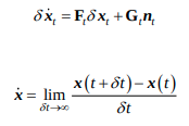
- 각 값들에 대한 delta는 다음식으로 계산된다. 그런데 코드상에서의 F와 아래 식에서의 F는 조금 다르다.
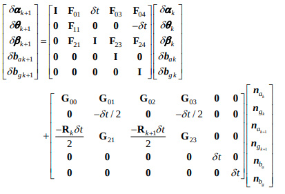
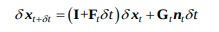
코드상에서의 F는 위식에서처럼 derivative가 적용되지 않은, 값들을 직접 구하는 것으로, 코드의 F = \(I+F_t\delta t\), V = \(G_t\delta t\)가 된다.
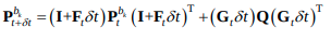
이후, 코드상에서의 jacobian과 covariance값은 다음식과 같이 계산된다.
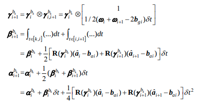
그에 따라 position, velocity, rotation의 preintegration 값들인 \(\alpha, \beta, \gamma\)는 다음식과 같이 계산될 것이다. (optimize 시에 사용되는 것으로 보인다.)
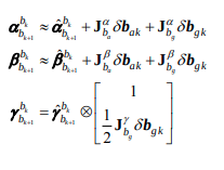
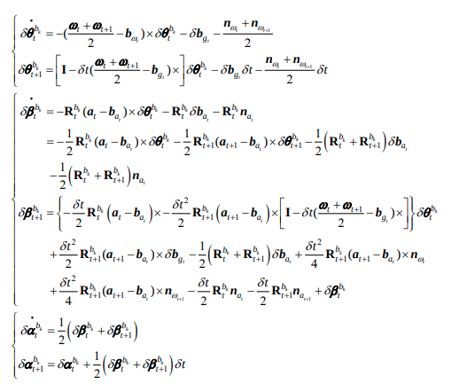
참고로 처음 \(\delta\)값은 위식으로부터 계산된 것이다. 자세한 내용은 Formula derivation pdf를 참고하자.
APPENDIX
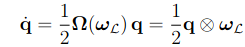
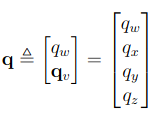
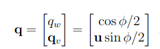
Quaternion은 다음과 같이 표현된다.
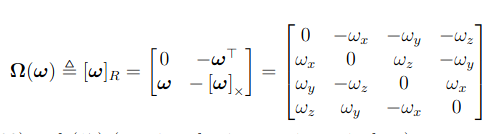
이때 쿼터니언과 각속도(\(\omega\))와의 관계를 알아보자.
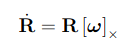
angular velocity를 rotation matrix로 위와 같이 표현 가능하다.
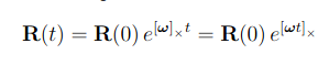

Taylor expansion을 적용하면, Rotation matrix는 위와 같이 표현 가능하다.
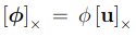
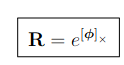
또한 cross-matrix의 성질과 Taylor expansion을 이용하면, Rotation matrix는
Rodrigue form으로 표현된다.
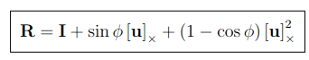
Rodrigues는 쿼터니안에서 위와같이 표현된다.
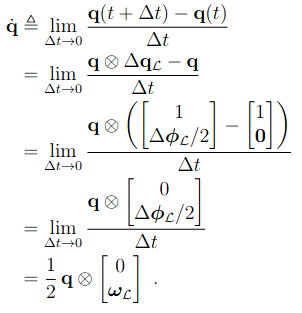
따라서 위식에서 pure quaternion부분은 \(\omega_L\)로 표현된다.
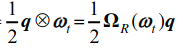
이때 quaternion의 곱은 다음과같이 계산되므로
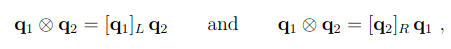
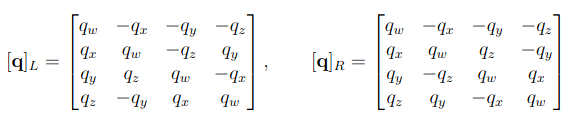
다음과 같은 연산자를 정의함으로써 마지막 식과 같이 \(\dot{q}\) 을 정의하게 된다.
VINS-Fusion 코드를 정리한 포스트입니다.
- VINS-Fusion Code Review - (1) Image Processing
- VINS-Fusion Code Review - (2) IMU Processing
- VINS-Fusion Code Review - (3) Initialization
- VINS-Fusion Code Review - (4) Sliding window & Optimization
- VINS-Fusion Code Review - (5) Marginalization
- VINS-Fusion Code Review - (6) Graph optimization
Reference
- [2017] Quaternion kinematics for the error-state Kalman filter.pdf
- [2005] Indirect Kalman Filter for 3D Attitude Estimation.pdf
- Formula Derivation and Analysis of the VINS-Mono.pdf
- Marginalization&Shcurcomplement.pptx
- [TRO2012] Visual-Inertial-Aided Navigation for High-Dynamic Motion in Built Environments Without Initial Conditions.pdf
- VINS-Mono.pdf